Mastering Infrastructure and Application Monitoring
Production Observability at Scale: Architectural Mechanics, Collection Topologies, and Time-Series Data Management
In modern, highly distributed software systems, running production workloads without robust observability is the engineering equivalent of flying a commercial airliner completely blind through a storm. As microservice ecosystems grow, cloud footprints scale dynamically, and ephemeral containerized infrastructure transforms infrastructure lifecycles, the traditional approaches to system monitoring break down. Determining that a system is merely 'up' or 'down' is no longer sufficient. Production issues present themselves as subtle degradations: a p99 latency spike in a downstream authentication service, a slow resource leak in an isolated container namespace, or an aggressive block-level disk write bottleneck inside a database cluster node.
To engineer a resilient system capable of sustaining self-healing autoscaling and deterministic multi-region fault tolerance, we must implement a multi-layered monitoring methodology. This discipline isolates the mechanical operating constraints of the underlying bare metal or virtualized compute resource from the internal behavior, logic, and state transitions of the execution runtimes. This comprehensive architectural manual deep-dives into the bifurcated paradigm of Infrastructure Monitoring versus Application Performance Monitoring (APM), exposes the core algorithmic collection engines that power enterprise monitoring tools, uncovers the mathematics of modern time-series compression, and maps out a production-grade blueprint for end-to-end telemetry systems.
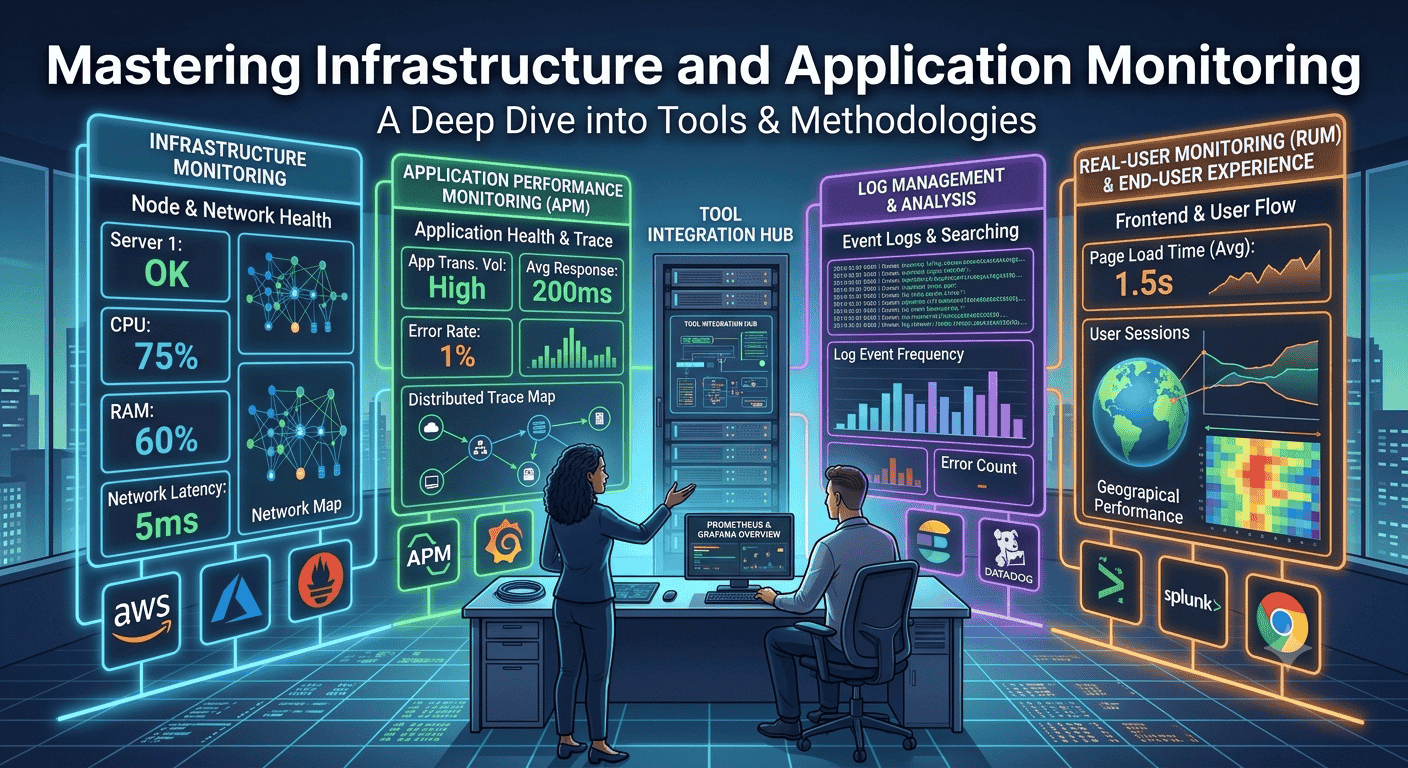
1. Paradigm 1: Deep-Dive Into Infrastructure Monitoring
Infrastructure Monitoring represents the foundational tier of system visibility. It treats the operating environment as a machine pool, observing the utilization, physical or logical hardware saturation, execution bottlenecks, and availability of resources regardless of what software process occupies the compute scope. Whether running on bare-metal hardware, local hypervisors (VMware, KVM), cloud EC2 instances, or orchestrated container nodes (Kubernetes kubelets), the objective remains uniform: preserve the hardware and OS execution platform so that runtime software can perform deterministically.
The Engineering Objective
The overriding objective of infrastructure monitoring is long-term capacity planning, predictive resource provisioning, hardware/OS fault isolation, and the elimination of runtime resource starvation. If an application crashes because the OS kernel runs completely dry of volatile memory or disk space, the failure is fundamentally an infrastructure management failure. Infrastructure metrics provide the raw telemetry data required by automated infrastructure controllers—such as cluster autoscalers or cloud hypervisor triggers—to dynamically provision compute capacity before the application tier experiences degraded execution environments.
Framework of Choice: The USE Method
Developed by legendary performance engineer Brendan Gregg, the USE Method serves as the industry standard for structural analysis of hardware and OS subsystems. For every logical and physical component in the host system (CPU, Memory, Network Interface, Disk Storage), engineers must evaluate three specific characteristics:
1. Utilization: The percentage of time that the resource was busy servicing work (e.g., CPU utilization sitting at 75%).
2. Saturation: The degree to which the resource has extra work that it cannot yet service, forcing tasks to sit in a waiting queue (e.g., CPU load averages exceeding the physical core count).
3. Errors: The absolute count of error events that occurred across the hardware or kernel subsystems (e.g., network packet drops or disk write retries).
Granular Metric Definitions and Technical Vectors
To implement effective infrastructure monitoring, DevOps teams must capture, track, and expose specific operating system and hardware counters:
* CPU Utilization & Throttling: Beyond simple usage tracking, we monitor `iowait` (the percentage of time the CPU sits idle waiting for disk or network I/O operations to complete) and `steal time` (the percentage of time a virtual CPU waits for the underlying physical hypervisor to allocate compute cycles, indicating a noisy neighbor problem in virtualized infrastructure). In containerized systems, we monitor CPU throttling metrics (`container_cpu_cfs_throttled_periods_total`), which reveal when the Linux kernel Completely Fair Scheduler (CFS) actively suppresses a process for exceeding its group limits.
* Memory Saturation and OOM Dynamics: Simple free memory monitoring is deeply deceptive because modern operating systems aggressively utilize unallocated RAM for page caching. Instead, engineers must monitor Available Memory (the RAM safely reclaimable without causing system slowdown) and Swap In/Out Rates. High swap-out rates imply active memory exhaustion. When host memory drops past a critical threshold, the kernel triggers the Out-Of-Memory (OOM) Killer, an OS mechanism that terminates high-scoring processes to prevent kernel panic. Monitoring the invocation logs of this system component (`kernel: Out of memory: Kill process`) is a critical production safety check.
* Disk Subsystem I/O and Queue Depth: Tracking remaining disk space storage capacity percentage is merely step one. High-throughput database systems demand deep observation of IOPS (Input/Output Operations Per Second), Disk Read/Write Latency, and Average Queue Depth. If disk latency spikes from 2ms to 200ms while disk space utilization is at only 40%, the system is suffering from physical I/O saturation, causing synchronous application execution threads to pool up and freeze.
* Network Interface Telemetry: This covers the physical or virtual network interface cards (NICs). Telemetry vectors include bandwidth utilization saturation (`tx_bytes` and `rx_bytes`), unaligned transmission framing anomalies, packet checksum mismatches, and dropped interface packets, which typically indicate a kernel ring buffer that is overflowing because the network soft-IRQ daemon cannot process network frame frames rapidly enough.
Production-Grade Alerting Policies
Alerts at this layer must be configured defensively to minimize pager fatigue while maintaining strong system safety guards:
* Alert 1: Storage Capacity Burn Rate (Warning Severity): Triggers if `disk_utilization_percentage > 85% AND predict_linear(disk_free_bytes[4h], 86400) < 0`. Rather than alerting statically on a fixed percentage, this linear regression formula predicts whether the storage volume will drop to 100% capacity within the next 24 hours based on the consumption slope over the last 4 hours. This shields engineers from waking up for static disks that sit permanently at 86% without changing.
* Alert 2: Node Unreachable / Heartbeat Timeout (Critical Severity): Triggers if `up{job="node-exporter"} == 0` for more than 2 minutes consecutively. This indicates that a host machine has dropped offline, suffered a hard freeze, or lost network access entirely, requiring immediate infrastructural failover or human intervention.
* Alert 3: Prolonged CPU Saturation (Warning Severity): Triggers if `node_load1 / count(node_cpu_seconds_total{mode="idle"}) > 1.5` sustained over 15 minutes. This mathematically determines that the system load queue contains 50% more active, execution-ready threads than the physical CPU core capacity can process concurrently, leading to system scheduling lag.
2. Paradigm 2: Deep-Dive Into Application-Level Monitoring (APM)
While infrastructure monitoring establishes the mechanical boundaries of the execution environment, Application Performance Monitoring (APM) pierces the black box of the operating system to witness what occurs inside the software application runtime itself. A virtual machine can report flawless metrics—15% CPU utilization, 20% memory usage, and zero disk latency—while the enterprise application it hosts is actively returning HTTP 500 internal server errors to 100% of incoming customer requests. APM fills this critical blindspot.
The Engineering Objective
The primary objective of application monitoring is the preservation of user experience, software execution correctness, business logic validation, and rapid root-cause isolation within distributed software microservices. APM enables developers and site reliability engineers (SREs) to track transactions across multi-layered dependencies, isolating failures down to a specific broken downstream service call, a locked SQL thread, or an unhandled null-pointer exception inside a specific code file module.
Framework of Choice: The RED Method & Golden Signals
For request-driven applications, industry standards focus heavily on the RED Method (popularized by Tom Wilkie) and Google’s Four Golden Signals. The core metrics encompass:
1. Rate / Throughput: The volume of raw demand being placed on the application engine, computed as inbound transactions or requests per second (RPS).
2. Errors: The absolute count or percentage ratio of transactions that fail to execute correctly, segmenting explicit software exceptions from standard business-logic responses.
3. Duration / Latency: The execution timeline tracking exactly how long it takes for requests to traverse the code stack and return responses to clients.
4. Saturation: A structural measure of how 'full' the application execution runtime is, looking at internal runtime limits like thread-pool depth or memory-heap allocation bounds.
Granular Metric Definitions and Technical Vectors
To construct an operational APM tier, application engines must instrument and export the following application-level variables:
* Mathematical Percentile Latencies (p50, p95, p99): In application performance monitoring, tracking average latency is a cardinal sin. Averages act as statistical masks that blend high performance with severe degradation. For instance, if 90 out of 100 users experience a lightning-fast response time of 50 milliseconds, but 10 users experience a catastrophic timeout of 10,000 milliseconds, the mathematical average reports a tolerable response time of roughly 1,000 milliseconds. This falsely indicates general health while 10% of the customer base suffers an outage. APM demands percentile tracking: p95 latency signifies that 95% of requests complete faster than the specified metric boundary, while p99 latency isolates the worst-performing 1% of transactions, exposing edge cases like database lock contention or severe memory garbage collection cycles.
* Error Rate Quantification: Application error tracking must be explicitly typed. We distinguish system failures (HTTP 5xx status codes, gRPC status codes like `INTERNAL` or `UNAVAILABLE`) from user-driven boundary failures (HTTP 4xx status codes, validation drops). Telemetry engines must compute the precise ratio of total errors to total inbound queries to generate a live, rolling error-rate percentage map.
* Application Runtime Saturation & Thread Dynamics: This tracks the concurrency limits of the software platform. In thread-per-request systems (e.g., traditional Java Tomcat deployments), engineers track Thread Pool Exhaustion (active threads versus max available worker threads). In single-threaded asynchronous loops (e.g., Node.js), observability targets Event Loop Lag—the delay between scheduling a callback function and its actual execution, indicating blocking synchronous computation. For memory-managed systems (Java, Go, .NET), metrics must record Garbage Collection (GC) Frequency and Pause Times, revealing when the application stops executing code to sweep dead memory allocations.
* Database Connection Pool Starvation: Modern applications leverage connection reuse pools to execute queries. If the application exhausts its maximum pool capacity, outbound transactions queue up internally waiting for a database socket connection to open up, triggering cascading request timeouts down the stack.
Production-Grade Alerting Policies
Alerting policies at the application layer are directly tied to Service Level Objectives (SLOs) and customer satisfaction parameters:
* Alert 1: High Error Rate Threshold (Critical Severity): Triggers if `sum(rate(http_requests_total{status=~"5.."}[5m])) / sum(rate(http_requests_total[5m])) * 100 > 2.0`. This calculation dynamically tracks the error ratio across a sliding 5-minute window. If structural HTTP 500 exceptions exceed 2% of total traffic, it signifies an active code failure or service disruption, requiring immediate notification to the on-call engineer.
* Alert 2: High Percentile Latency Degradation (High Severity): Triggers if `histogram_quantile(0.95, sum(rate(http_request_duration_seconds_bucket[5m])) by (le)) > 2.0` for 3 consecutive execution cycles. This PromQL expression calculates the 95th percentile latency of the system. If 5% of users are experiencing response wait times exceeding 2.0 seconds over a prolonged period, the system triggers a remediation event.
* Alert 3: Database Connection Pool Exhaustion (Warning Severity): Triggers if `app_db_connections_active / app_db_connections_max > 0.85` sustained for more than 60 seconds. This predictive trigger identifies upcoming application starvation before connections run dry and halt request execution.
3. The Architectural Mechanics of Pull-Based Collection
The architectural mechanisms that govern how metrics migrate from an application execution space to a central monitoring cluster define the scalability limits of your operational system. For decades, traditional enterprise software relied on the Push-based model. Under this paradigm, every host machine or application run tier embeds a stateful monitoring agent. This agent tracks metrics locally and initiates outbound TCP connections to blast that data over the network to a central storage system or load-balanced collector array. While intuitive, this approach presents major performance bottlenecks in elastic, high-concurrency cloud environments. This structural bottleneck led to the development of the Pull-based model, engineered as a core design principle of the Cloud Native Computing Foundation (CNCF) monitoring stack.
The Mechanics of the Pull Model
In a pure pull-based monitoring topology, such as Prometheus, the relationship between the application target and the monitoring engine is completely inverted. The monitored application or compute instance remains entirely passive regarding metrics delivery. It does not know where the monitoring cluster resides, nor does it attempt to push network frames over the wire.
Instead, the application runs a lightweight, hyper-efficient embedded HTTP server that exposes a single public endpoint, almost universally bound to the path `/metrics`. When internal code events occur (e.g., an API route executes), the application updates simple memory counters sitting in local RAM. When the central monitoring server executes its scrape interval loop, it initiates an inbound HTTP `GET` request to the target, consumes the raw plain-text payload containing the metric states, and closes the connection.
The Plain-Text Metric Format
The data transmitted during a scrape event is explicitly structured using standard line-oriented plain text. This human-readable format became the foundation for the open-source industry standard known as OpenTelemetry (OTel) and OpenMetrics. The structure looks like this:
# HELP http_requests_total Total number of HTTP requests processed.# TYPE http_requests_total counterhttp_requests_total{method="POST",handler="/api/v1/checkout",status="200",env="prod"} 14205http_requests_total{method="POST",handler="/api/v1/checkout",status="500",env="prod"} 12# HELP node_memory_Active_bytes Memory actively in use by the OS kernel.# TYPE node_memory_Active_bytes gaugenode_memory_Active_bytes{instance="node-1.internal",zone="us-east-1a"} 68719476736Why Pull Models Win in Cloud-Native and Kubernetes Environments
The pull-based architecture offers distinct operational advantages over push configurations in high-density, dynamic auto-scaling clusters:
1. Isolation of Resource Cost Under Heavy Load: Consider a scenario where an application microservice undergoes a massive traffic spike, scaling from 1,000 requests per second to 100,000 requests per second. In a push-based model, the monitoring agent attempts to generate and push 100,000 metric payloads across the network to the central engine. This extra compute and I/O load can starve the app of resources, compounding the outage. In contrast, with a pull model, the application simply increments an in-memory counter variable. The memory and CPU footprint remain completely flat. Prometheus continues to pull data at its pre-configured interval (e.g., once every 15 seconds), cleanly separating application load from telemetry delivery costs.
2. Native Service Discovery Integration: In elastic container environments like Kubernetes, workloads are highly ephemeral. Pods spin up, receive random dynamic internal IP addresses, execute for minutes or hours, and terminate. A monitoring system cannot rely on static lists of IP addresses. Prometheus bridges this gap by integrating directly with the Kubernetes API server. It listens continuously to the cluster state, discovering pods as they register with the API. It evaluates custom Kubernetes annotations on the pods to dynamically determine which endpoints to scrape, what port to target, and how frequently to collect data—completely eliminating manual configuration overhead.
3. Elimination of Central Ingestion Flood Management: In a push-based environment, if 5,000 containers suddenly reboot simultaneously after a bad deployment, they will all aggressively attempt to establish network connections to push their boot metrics to the central metrics collector. This can create a massive distributed denial of service (DDoS) effect that crashes the monitoring infrastructure. In a pull network, the monitoring cluster retains total control over its network ingestion queues. It orchestrates its scrape intervals smoothly, pacing outbound requests to match its internal processing limits.
4. Deep-Dive Into Time-Series Database (TSDB) Storage Engines
Once a monitoring engine scrapes data from thousands of targets across an enterprise network, it faces a daunting data ingestion challenge: processing millions of concurrent incoming data metrics every second and storing them in a format that allows real-time mathematical querying. Traditional relational database management systems (RDBMS) like PostgreSQL or MySQL fail completely at this task. They are bound by write locks, heavy indexing schemas, and row-level write amplification that chokes under high-volume streaming data. This architectural challenge drove the engineering of custom Time-Series Databases (TSDB).
The Anatomy of a Time-Series Metric
A time-series metric represents a sequence of data points indexed entirely by chronological order. In the Prometheus TSDB subsystem, a specific time series is uniquely identified by its coordinate dimensions, separating the identifier from the chronological telemetry line:
Series Identity = Metric Name + Unique Combination of Key-Value LabelsExample:http_requests_total{method="GET", status="200"} -> Series ID #74105Chronological Telemetry Stream for Series ID #74105:(timestamp_1, value_1) -> (1719878400, 42.0)(timestamp_2, value_2) -> (1719878415, 46.0)(timestamp_3, value_3) -> (1719878430, 51.0)The metric values are universally stored as 64-bit IEEE 754 floating-point numbers, while the timestamps are tracked as 64-bit Unix epochs in milliseconds.
The Write Pipeline: Head Blocks and Write-Ahead Logs (WAL)
To achieve high-frequency write speeds, a TSDB avoids immediate disk commits. The ingestion engine operates an in-memory buffer called the Head Block:
1. The Ingestion Path: When a new metric value is collected, it is appended to an in-memory data structure inside the Head Block. This allows fast memory writes without disk I/O bottlenecks.
2. The Write-Ahead Log (WAL): Because memory is volatile, a sudden power failure or system crash would lose all buffered data in the Head Block. To guarantee durability, the incoming data point is simultaneously appended to an on-disk, append-only file called the Write-Ahead Log (WAL). This write is highly efficient because it requires no structural indexing; it is a raw append to the end of a physical file descriptor on disk. If the server crashes, the engine replays the WAL on boot to rebuild the in-memory Head Block state.
Data Compaction and the Gorilla Compression Algorithm
Every 2 hours, the TSDB takes the accumulated data within the in-memory Head Block, freezes it, and writes it to permanent disk storage as an immutable data block containing an index file and raw chunk directories. To prevent this data from consuming terabytes of storage space, the TSDB employs highly specialized bit-level data compression algorithms, heavily based on the Facebook Gorilla TSDB architecture.
The database uses two distinct compression schemas for timestamps and floating-point values:
* Timestamp Compression via Delta-of-Deltas: In regular production monitoring, scrapes happen at highly predictable intervals (e.g., exactly every 15 seconds). This means the difference (delta) between consecutive timestamps is almost always constant. For example, given a sequence of timestamps $T_1, T_2, T_3$: if $T_2 - T_1 = 15,000$ milliseconds, and $T_3 - T_2 = 15,000$ milliseconds, the delta-of-deltas is exactly $(T_3 - T_2) - (T_2 - T_1) = 0$. Instead of storing a full 64-bit timestamp, the Gorilla engine stores a single bit `0`. If the scrape interval varies slightly (e.g., due to minor network latency), the delta-of-deltas will be a small number. The algorithm then outputs a specialized bit header prefix followed by just a few bits representing the minor variance. This technique allows timestamps to consume an average of only 1.37 bytes per data point, achieving a massive compression ratio.
* Value Compression via XOR Bitwise Manipulation: Floating-point values (like CPU utilization percentages) often change very little from one scrape to the next (e.g., going from 54.21% to 54.22%). The Gorilla engine compresses these values by performing a bitwise XOR operation between the current floating-point value and the preceding value. If the values are identical, the XOR result is zero, which is stored as a single bit `0`. If the values differ slightly, the XOR operation exposes that only a small, localized sequence of bits in the middle of the 64-bit structure has changed (with leading and trailing zeros). The engine discards the unchanging leading and trailing zeros, records a flag detailing the bit offset bounds, and stores only the modified bits. This reduces the average storage footprint of a 64-bit float down to just a few bits under steady-state operation.
5. Comparative Technical Analysis: Tooling Architecture Matrix
Selecting a modern monitoring stack requires navigating complex architectural trade-offs across collection protocols, storage limits, network topologies, and cost boundaries. The following architectural matrix provides an end-to-end technical breakdown of the industry's leading monitoring paradigms.
| Architectural Dimension | Cloud-Native (Prometheus / Grafana Stack) | Enterprise Unified SaaS (Datadog, New Relic) | Legacy Data Center (Zabbix, Nagios Core) |
|---|---|---|---|
| Data Collection Model | Pure Pull Architecture. Central server initiates inbound HTTP/HTTPS connections to scrapable endpoints. | Hybrid Push Model. Local background daemons aggregate data and stream outbound HTTPS telemetry payloads. | Agent-Driven Push or Synchronous ICMP/SNMP poll loops executed against target configurations. |
| Core Storage Engine | Local ephemeral single-node TSDB. Optimized for raw ingestion speed and short retention windows. | Globally distributed multi-tenant columnar cloud data lakes with automated cold/hot tiering policies. | Traditional relational databases (PostgreSQL/MySQL) with complex custom schema partitions. |
| Network Footprint | Inbound-heavy topology. Requires clear network access vectors from the collection server to application namespaces. | Outbound-only footprint. Ideal for tightly restricted firewalls; demands zero inbound port openings. | Heavy continuous internal network chatter via stateful TCP agent sockets or synchronous ping sweeps. |
| Cardinality Boundaries | High-cardinality vulnerability. Unique or random label values (e.g., user IDs) inflate memory state and degrade TSDB speed. | Managed high cardinality. SaaS index structures absorb complex label dimensions but apply steep cost penalties. | Extremely rigid. Adding metadata parameters requires explicit table schema adjustments, capping flex options. |
| Long-Term Archiving | Requires secondary replication blocks (Thanos, Cortex, Mimir) to stream immutable data segments to cloud object storage. | Built-in natively. Retains historical metrics for months or years based on tiering agreements. | Relies entirely on database backup procedures, database clustering, or physical storage array scaling. |
6. Engineering the Long-Term Retention Challenge: Thanos & Mimir
Because the Prometheus TSDB engine was built for high-speed local processing, it stores metrics directly on the local non-volatile storage attached to the host server container. This intentional design choice isolates the monitoring system from external network storage dependencies when evaluating alerts. However, it introduces a major architectural limitation: the local server cannot scale infinitely. Attempting to store years of historical telemetry data on a single local drive eventually runs out of disk space, makes query times unmanageably slow, and creates a single point of failure if the disk corrupts.
To resolve this constraint while preserving open-source architectures, the cloud-native ecosystem relies on secondary scaling systems like Thanos or Grafana Mimir. These tools sit alongside Prometheus to enable high-availability clustering and long-term historical retention.
The Sidecar Archiving Architecture
Thanos addresses this by deploying a lightweight Sidecar agent directly inside the same pod or virtual machine where the Prometheus server executes. This architecture operates through a clear decoupling of hot and cold data tiers:
1. Local Scrape and Hot Retention: Prometheus continues to scrape endpoints locally and write data points to its internal Head Block every 2 hours, exactly as before. It retains a brief local history (e.g., 24 to 48 hours) to service real-time local alerting queries.
2. Cold Tier Shipping: The moment Prometheus finishes sealing a 2-hour immutable TSDB block onto local disk, the Thanos Sidecar intercepts the event. It picks up the block, applies additional compression, and uploads the immutable file structures across the network to an inexpensive, durable cloud object storage system, such as AWS S3, Google Cloud Storage (GCS), or an on-premises MinIO cluster.
The Store-Gateway Query Execution Path
When an SRE opens a Grafana dashboard and requests a metric visualization covering the past 12 months, the query engine no longer hits the local Prometheus instance. Instead, the query routes to a component called the Thanos Querier or a centralized Mimir Query Frontend.
This query subsystem reads metadata from across the topology and splits the query execution path into two parallel streams:
* The Hot Path: It queries the active, real-time Prometheus instances directly to gather the freshest metrics covering the last few hours.
* The Cold Path: It contacts a set of distributed proxies called Thanos Store Gateways. These gateways pull only the highly compressed historical index blocks required from the cloud object storage bucket, evaluating the historical time ranges in parallel.
The query engine merges these two streams into a single, seamless data timeline, providing the developer with historical analysis across years of data while keeping local Prometheus storage requirements completely lightweight and safe from disk exhaustion.
7. The Production Observability Readiness Checklist
Before signing off on any production deployment, platform engineering teams should validate that their monitoring setup can withstand major infrastructure stress. Run through this engineering checklist to ensure your system is fully resilient:
* [ ] Validate Scrape Timelines against Target Timeouts: Verify that the Prometheus scrape timeout configuration is strictly less than the scrape interval (e.g., timeout at 10 seconds for a 15-second interval). This prevents network connectivity locks from piling up outstanding scrape loops.
* [ ] Enforce Explicit Cardinality Limiters: Ensure that no application code generates high-cardinality label variables dynamically. Check that random data inputs, such as raw UUIDs, email addresses, or unmasked credit card tokens, are never injected into metric labels, as this will rapidly bloat TSDB memory structures.
* [ ] Verify Multi-AZ Monitoring Redundancy: Ensure your monitoring infrastructure is not cross-dependent on the zones it observes. Deploy Prometheus collectors across distinct availability zones, and run alerting managers in independent fault domains to guarantee alerts still fire during regional network splits.
* [ ] Implement automated synthetic check routines: Deploy simple black-box monitoring runtimes to continuously perform synthetic HTTP handshakes against primary entry gateways. This provides an independent validation loop that mimics real user journeys alongside your internal telemetry.